はじめましてフバチと申します。私は、もともと化学エンジニアで、日本に来る前は、ワルシャワ工科大学(ポーランド)で20年ほど働いていました。私は2021年5月からエコモットのデータアナリティクス部に勤務しています。エコモットで働くことで、異常検知、点群超解像、画像ノイズ除去といった問題に対するAI手法の応用について、新たな経験を積むことが出来ました。これらの問題はすべて、私にとって非常に興味深いものでした。また、私自身、化学工学の課題にAIツールを導入することにも興味があり、最近、物理情報に基づくニューラルネットワーク(PINN)について調べています。
このブログでは、私が調査したPINNについて、簡単な実験を交えて紹介したいと思います。データ分析やAI活用に興味がある方から反応を頂ければ嬉しく思います。
PINNは、物質、エネルギー、流体などの輸送現象のシミュレーションを可能にします。このようなシミュレーションは、化学反応におけるプロセス理解には欠かせません。
物理情報ニューラルネットワーク(PINN)
PINNは、科学的問題を解決するツールとしてRaissi et al.(2017a), Raissi et al.(2017b), Raissi et al.(2019)によって紹介されています。このような問題は通常、偏微分方程式(PDE)または常微分方程式(ODE)を用いて記述できる物理法則によって支配されている。そのため、PINNの構造は、所望のODEまたはPDE系を統合するように設計されています。このため、PINNの学習時には、さらなる制約が課されます。それらの制約条件は、PDEやODEの形式だけでなく、境界条件や初期条件からも生じます。さらに、これらの制約は、学習したニューラルネットワークに新たな情報を提供します。そのため、実験データの必要性が減り、境界条件や初期条件の値だけで、問題を解くことも可能になるのです。
以下、流れのシミュレーションに関する調査と簡単な実験を行いましたので、読んでいただければ幸いです。(英語で申し訳ありません。)
Application of PINN
- Simulation of the phenomenon (i.e., profiles prediction of velocity, temperature, component concentration etc. using calculations) (Raissi et al., 2017a). This kind of calculation can be performed using only boundary and initial conditions. However, the availability of experimental data will improve the accuracy of the simulation.
- Use of PINN for inverse estimation of physical properties from measured experimental data (Raissi et al., 2017b).
- Discovery of the form of governing partial differential equations from experimental data (Chen et al., 2021).
PINN for flow simulation
In the literature it can be found at least two different approaches to flow simulation using PINN:
Approach 1: PINN for solving Navier-Stokes equation in the case of 2D incompressible fluid flow introduced by Raissi et al. (2017b). Let’s call it traditional PINN. The authors applied stream function to automatically satisfy the continuity equation. Hence, in this approach neural networks were used for the estimation of the values of pressure and stream function(p,Ψ). Subsequently, velocity vector was calculated using the stream function.
Approach 2: Mix-variable PINN introduced by Rao et al. (2020). The authors wanted to avoid second order derivatives in PDE. This was achieved by introducing Cauchy stress tensor into their model. Consequently, neural networks were used for the estimation of the values of pressure, stream function and the Cauchy stress tensor(p,Ψ,σ)(Fig.2). The authors claimed that in this way the trainability and accuracy of the model was improved.
Application of PINN for the simulation of flow between two parallel plates
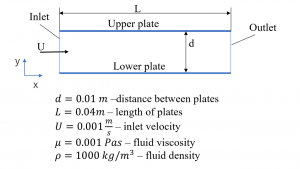 Fig. 1. Flow between two plates: the geometry and the values of the parameters.
PINN was applied to simulate the fluid velocity during the steady and incompressible flow between two parallel and horizontal plates. The geometry of the flow and the values of the other operating parameters are shown in the Fig.1. As it can be seen in this figure flow was treated as 2D. This means that the changes in velocity along the second horizontal direction was neglected. It should be mentioned, that in this case the profile of the x component of velocity vector can be also obtained analytically if considering the region sufficiently far from the inlet.
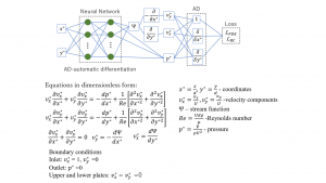 Fig. 2. Traditional PINN for the simulation of flow between two plates.
The flow between two plates was simulated using both traditional and mix-variable PINNs of which architectures and the PDEs forms are shown in Fig. 2 and Fig. 3 respectively. As it can be seen in these figures mix-variable PINN model needed more equations than traditional PINN model. However, mix-variable PINN model did not contain second order derivatives. Additionally, both models were implemented using SciANN (Haghighat and Juanes, 2021) a Python package for PINN application, which was built based on Tensorflow and Keras. Thus, it inherited many of Kera’s functionalities.
The calculation was conducted for 6 different cases of which details are shown in Table 1. Moreover, the default SciANN setting was kept for the other parameter not shown in this table (e.g. loss_func: “mse”, optimizer: “adam”).
In Table 1, there are also shown the total number of colocation points (i.e., the points for which PINN calculated flow parameters) and the number of those point in x and y directions (in the bracket). During these calculations, those points were regularly distributed in the space between two plates.
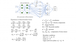 Fig. 3. Mix-variable PINN for the simulation of flow between two plates.
The example of simulation results is shown in Fig.4. The distribution of velocity and pressure along the space between two plates can be seen in Fig. 4a. On the other hand, the comparison of PINN calculation with analytical solution is given in Fig. 4b. These results indicated that velocity profile developed relatively quickly and after that there was a good agreement between PINN result and analytical solution. Similar results were obtained for all considered cases (see Table 1).
The additional results of simulation are shown in Table 2. This table contains the values of average axial velocities vx* , which were calculated using x velocity components along the axis y at the given distance from the inlet. Because of the inlet boundary condition (see Fig. 2 and 3), it was expected that vx*=1. Nevertheless, due to the computational error the values of vx* are smaller than one. This discrepancy between expected and calculated value was smaller in the case of mix-variable PINN model than in the case of traditional PINN model. Similarly, when the number of colocation points was increased vx* become closer to 1.
In Table 2 there are also shown the values of loss function for each of the studied cases. The loss function was smaller in the case of mix-variable PINN model and its value decreased when the number of colocation points increased.
To conclude, it seems that Rao et al. (2020) was right that the rejection of second derivatives from PDE improves trainability and accuracy of the model. Nevertheless, my results also indicated that performance of PINN depends on the number of colocation points.
Table 1. The PINN architecture, training pattern and the number of colocation points.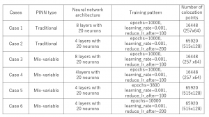
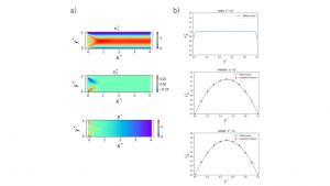 Fig. 4. The example of simulation results obtained using mix-variable PINN (case 6): a) distribution of velocity and pressure in the space between two plates; b) velocity profile at the given distance from the inlet.
Table 2. The results of simulation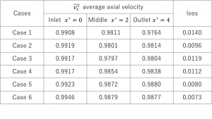
Application of PINN for the simulation of flow between two concentric cylinders with rotating inner one
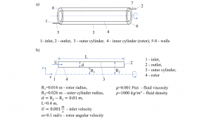
Fig. 5. Flow between two concentric cylinders with rotating inner one: a) reactor with such a flow; b) 2D approximation – black contours shows the space between cylinders where the fluid flows.
Flow between two concentric cylinders with rotating inner one (rotor) is illustrated in Fig. 5. This flow is 3D (Fig 5a), however, at sufficiently low rotor rotation its geometry can be simplified as shown in Fig. 5b. This simplification requires assumption that the values of all derivatives in angular direction are zeros (this means that pressure and velocity can change values only in x and r direction). Under such an assumption this flow can be approximated using axisymmetric swirl model (see for example ANSYS FLUENT 12.0/12.1 Documentation). This model is not really 2D because although derivatives of pressure and velocity in angular direction disappear the angular component of velocity is still calculated.
Application of axisymmetric swirl model requires transformation of governing PDEs into cylindrical coordinate form. My previous attempts of simulation of the flow in a pipe using equations in cylindrical coordinates showed poor performance of traditional and mix-variable PINNs. Therefore, I decided to use neural networks for the estimation of the values of pressure and velocity components(p, vx, vr, vθ). As the result, the form of PDEs and PINN architecture used for these simulations were as illustrated in Fig. 6.
The calculation was conducted for 4 different cases of which details are shown in Table 3. Meanwhile, the values of axial and rotor angular velocity were chosen to be small enough (see Fig. 5 b) so that velocity components could be calculated analytically for the region sufficiently far from the inlet.
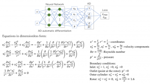
Fig. 6. PINN for the simulation of flow between two concentric cylinders with rotating inner one.
The example of simulation results is shown in Fig.7. The distribution of velocity and pressure along the space between two cylinders can be seen in Fig. 7a. Meanwhile, in Fig. 7b and 7c the comparison of PINN calculations with analytical solutions are given. These results indicated that velocity profile developed relatively quickly in the case of axial velocity. On the contrary, in the case of angular velocity the discrepancy between simulation and analytical solution was significant for the wider distance from the inlet. Similar results were obtained for all considered cases (see Table 3).
The values of average axial velocities vx* and loss function are shown in Table 4. Similarity to the flow between two plates the discrepancy between expected (which should be also 1) and calculate vx* were noticed. This discrepancy as well as loss function became smaller when number of colocation points was increased.
Table 3. The neural network architecture, training pattern and the number of colocation points.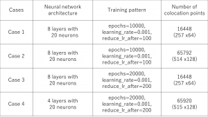
Table 4. The results of simulation
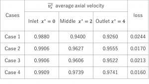
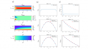
Fig. 7. The example of simulation results (case 4): a) distribution of velocity and pressure in the space between two cylinders; b) axial velocity (vx) profile at the given distance from the inlet; c) angular velocity (vθ) profile at the given distance from the inlet.
In conclusion, it seems that if the PDEs have cylindrical coordinate form better results could be obtained when velocity vector is estimated directly by neural networks (i.e., without stream function). Moreover, similarly to the flow between two plates the accuracy of the prediction increases with the increasing in the number of colocation points.
Literature:
Chen Z., Liu Y., Sun H. (2021): Physics-informed learning of governing equations from scarce data. Nat Commun 12, 6136.
Haghighat E, Juanes R. (2021): SciANN: A Keras/Tensorflow wrapper for scientific computations and physics-informed deep learning using artificial neural networks. Computer Methods in Applied Mechanics and Engineering, 373.
Raissi, M., Perdikaris, P., and Karniadakis, G. E. (2017a): Physics informed deep learning (part i): Data-driven solutions of nonlinear partial differential equations. arXiv preprint arXiv:1711.10561.
Raissi, M., Perdikaris, P., and Karniadakis, G. E. (2017b): Physics informed deep learning (part ii): Data-driven discovery of nonlinear partial differential equations. arXiv preprint arXiv:1711.10566.
Raissi, M., Perdikaris, P., and Karniadakis, G. E. (2019): Physics-informed neural networks: A deep learning framework for solving forward and inverse problems involving nonlinear partial differential equations. Journal of Computational Physics 378, 686–707
Rao C., Sun H., Liu Y., (2020): Physics-informed deep learning for incompressible laminar flows. Theoretical and Applied Mechanics Letters,vol. 10, 3, 207–212.